3. KNN
K-Nearest Neighbors (KNN) is a simple, versatile, and non-parametric machine learning algorithm used for classification and regression tasks. It operates on the principle of similarity, predicting the label or value of a data point based on the majority class or average of its k nearest neighbors in the feature space. KNN is intuitive and effective for small datasets or when interpretability is key.
Key Concepts
-
Instance-Based Learning: KNN is a lazy learning algorithm, meaning no explicit training phase is required. It stores the entire dataset and performs calculations at prediction time.
-
Distance Metric: The algorithm measures the distance between data points to identify the nearest neighbors. Common metrics include:
Metric Formula Euclidean distance \( \displaystyle \sqrt{\sum_{i=1}^n (x_i - y_i)^2} \) Manhattan distance \( \displaystyle \sum_{i=1}^n \|x_i - y_i\| \) Minkowski distance \( \displaystyle \left( \sum_{i=1}^n \|x_i - y_i\|^p \right)^{1/p} \) -
K Value: The number of neighbors considered. A small k can be sensitive to noise, while a large k smooths predictions but may dilute patterns.
-
Decision Rule:
- Classification: The majority class among the k neighbors determines the predicted class.
- Regression: The average (or weighted average) of the k neighbors' values is used.
Mathematical Foundation
KNN relies on distance calculations to find neighbors. For a data point \( x \), the algorithm: 1. Computes the distance to all points in the dataset using a chosen metric (e.g., Euclidean distance). 2. Selects the k closest points. 3. For classification, assigns the class with the most votes among the k neighbors. For regression, computes the mean of their values.
Example: Classification
Given a dataset \( D = \{(x_1, y_1), (x_2, y_2), ..., (x_n, y_n)\} \), where \( x_i \) is a feature vector and \( y_i \) is the class label, predict the class of a new point \( x \):
- Calculate distances \( d(x, x_i) \) for all \( i \).
- Sort distances and select the k smallest.
- Count the class labels of these k points and assign the majority class to \( x \).
Weighted KNN
In weighted KNN, neighbors contribute to the prediction based on their distance. Closer neighbors have higher influence, often weighted by the inverse of their distance:
For regression, the prediction is:
Visualizing KNN
To illustrate, consider a 2D dataset with two classes (blue circles and red triangles). For a new point (green star), KNN identifies the k nearest points and assigns the majority class.

Figure: KNN with k=3. The green star is classified based on the majority class (blue circles) among its three nearest neighbors.
For regression, imagine predicting a continuous value (e.g., house price) based on the average of the k nearest houses’ prices.
Plot: Decision Boundary
KNN’s decision boundary is non-linear and depends on the data distribution. Below is an example of decision boundaries for different k values:
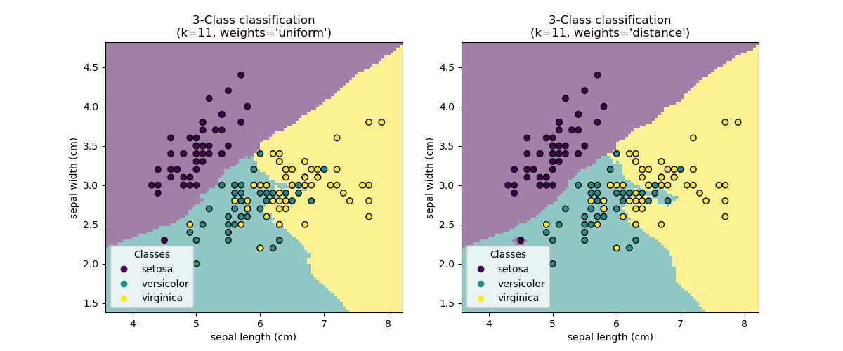
Figure: Decision boundaries for k=1, k=5, and k=15. Smaller k leads to more complex boundaries, while larger k smooths them.
Pros and Cons of KNN
Pros
- Simplicity: Easy to understand and implement.
- Non-Parametric: Makes no assumptions about data distribution, suitable for non-linear data.
- Versatility: Works for both classification and regression.
- Adaptability: Can handle multi-class problems and varying data types with appropriate distance metrics.
Cons
- Computational Cost: Slow for large datasets, as it requires calculating distances for every prediction.
- Memory Intensive: Stores the entire dataset, which can be problematic for big data.
- Sensitive to Noise: Outliers or irrelevant features can degrade performance.
- Curse of Dimensionality: Performance drops in high-dimensional spaces due to sparse data.
- Choosing K: Requires careful tuning of k and distance metric to balance bias and variance.
KNN Implementation
Below are two implementations of KNN: one from scratch and one using Python’s scikit-learn library.
From Scratch
This implementation includes a basic KNN classifier using Euclidean distance.
Accuracy: 1.00
import numpy as np
from sklearn.datasets import make_classification
from sklearn.model_selection import train_test_split
from sklearn.metrics import accuracy_score

class KNNClassifier:
    def __init__(self, k=3):
        self.k = k

    def fit(self, X, y):
        self.X_train = X
        self.y_train = y

    def predict(self, X):
        predictions = [self._predict(x) for x in X]
        return np.array(predictions)

    def _predict(self, x):
        # Compute Euclidean distances
        distances = [np.sqrt(np.sum((x - x_train)**2)) for x_train in self.X_train]
        # Get indices of k-nearest neighbors
        k_indices = np.argsort(distances)[:self.k]
        # Get corresponding labels
        k_nearest_labels = [self.y_train[i] for i in k_indices]
        # Return majority class
        most_common = max(set(k_nearest_labels), key=k_nearest_labels.count)
        return most_common

# Example usage

# Generate synthetic dataset
X, y = make_classification(n_samples=100, n_features=2, n_informative=2, n_redundant=0, n_repeated=0, n_classes=2, n_clusters_per_class=1, random_state=42)
X_train, X_test, y_train, y_test = train_test_split(X, y, test_size=0.2, random_state=42)

# Train and predict
knn = KNNClassifier(k=3)
knn.fit(X_train, y_train)
predictions = knn.predict(X_test)
print(f"Accuracy: {accuracy_score(y_test, predictions):.2f}")
Using Scikit-Learn
Accuracy: 1.00
import numpy as np
import matplotlib.pyplot as plt
from io import StringIO
from sklearn.datasets import make_classification
from sklearn.model_selection import train_test_split
from sklearn.neighbors import KNeighborsClassifier
from sklearn.metrics import accuracy_score
import seaborn as sns

plt.figure(figsize=(12, 10))

# Generate synthetic dataset
X, y = make_classification(n_samples=100, n_features=2, n_informative=2, n_redundant=0, n_repeated=0, n_classes=2, n_clusters_per_class=1, random_state=42)
X_train, X_test, y_train, y_test = train_test_split(X, y, test_size=0.2, random_state=42)

# Train KNN model
knn = KNeighborsClassifier(n_neighbors=3)
knn.fit(X_train, y_train)
predictions = knn.predict(X_test)
print(f"Accuracy: {accuracy_score(y_test, predictions):.2f}")

# Visualize decision boundary
h = 0.02  # Step size in mesh
x_min, x_max = X[:, 0].min() - 1, X[:, 0].max() + 1
y_min, y_max = X[:, 1].min() - 1, X[:, 1].max() + 1
xx, yy = np.meshgrid(np.arange(x_min, x_max, h), np.arange(y_min, y_max, h))

Z = knn.predict(np.c_[xx.ravel(), yy.ravel()])
Z = Z.reshape(xx.shape)

plt.contourf(xx, yy, Z, cmap=plt.cm.RdYlBu, alpha=0.3)
sns.scatterplot(x=X[:, 0], y=X[:, 1], hue=y, style=y, palette="deep", s=100)
plt.xlabel("Feature 1")
plt.ylabel("Feature 2")
plt.title("KNN Decision Boundary (k=3)")

# Display the plot
buffer = StringIO()
plt.savefig(buffer, format="svg", transparent=True)
print(buffer.getvalue())

plt.close()
Exercício
 16.sep
  23:59
23:59Dentre os datasets disponíveis, escolha um cujo objetivo seja prever uma variável categórica (classificação). Utilize o algoritmo de KNN para treinar um modelo e avaliar seu desempenho.
Utilize as bibliotecas pandas, numpy, matplotlib e scikit-learn para auxiliar no desenvolvimento do projeto.
A entrega deve ser feita através do Canvas - Exercício KNN. Só serão aceitos links para repositórios públicos do GitHub contendo a documentação (relatório) e o código do projeto. Conforme exemplo do template-projeto-integrador. ESTE EXERCÍCIO É INDIVIDUAL.
A entrega deve incluir as seguintes etapas:
| Etapa | Critério | Descrição | Pontos |
|---|---|---|---|
| 1 | Exploração dos Dados | Análise inicial do conjunto de dados - com explicação sobre a natureza dos dados -, incluindo visualizações e estatísticas descritivas. | 20 |
| 2 | Pré-processamento | Limpeza dos dados, tratamento de valores ausentes e normalização. | 10 |
| 3 | Divisão dos Dados | Separação do conjunto de dados em treino e teste. | 20 |
| 4 | Treinamento do Modelo | Implementação do modelo KNN. | 10 |
| 5 | Avaliação do Modelo | Avaliação do desempenho do modelo utilizando métricas apropriadas. | 20 |
| 6 | Relatório Final | Documentação do processo, resultados obtidos e possíveis melhorias. Obrigatório: uso do template-projeto-integrador, individual. | 20 |